> For the complete documentation index, see [llms.txt](https://hapi-one.gitbook.io/hapi-protocol/llms.txt). Markdown versions of documentation pages are available by appending `.md` to page URLs; this page is available as [Markdown](https://hapi-one.gitbook.io/hapi-protocol/hapi-core-of-decentralized-cybersecurity/machine-learning.md).
# Machine Learning
The utilization of machine learning algorithms is immensely useful in different aspects of data categorization. Categorization or classification algorithm is able to achieve exactly what HAPI Protocol needs - less computational overhead which also means increased data processing and higher specificity and accuracy of detection. At this juncture, pattern recognition is a crucial aspect of identifying the transactional history of an address, ramifications of the transaction paths, and commonalities in behavior. These similarities in behavior are specifically what we are interested in since they will, potentially, enable HAPI Protocol to operate at almost instantaneous speeds, allocating even more time for entities using HAPI to act on the illicit activity.
The complex issue arises when there is a need to utilize machine learning but there is not sufficient data on fraudulent transactions, for that reason, the first iteration of machine learning implementation will have a binary classification algorithm that will only have two potential predictors 0 or 1.
1 - identifies that the transaction in question is in fact fraudulent or poses a potential risk and 0 - refers to a safe risk score.
The core of the model then is created using customary variables, for the sake of simplicity and visualization, we will use 10 common variables: block\_timestamp, block\_n\_txs, n\_inputs, input\_sum, output\_sum, n\_outputs, output\_seq, and input\_seq. These will represent the base of the model. However, in order to refine and increase the accuracy of the baseline, we will need to employ a feature engineering technique that will help to achieve both granularities in classification and lay the foundation for model building.
Although the Supervised model of machine learning is ideal for our use since our model possesses a specific dataset, it is fraught with one issue in our case that may hinder accurate prediction - overfitting. The issue lies in the overdependence of the model on the very same predetermined datasets on which the model is being trained. To rectify overfitting issues effectively we need to apply a cross-validation workflow. In essence, cross-validation allows us to experiment on the independent dataset while holding out the test data enabling an effective partitioning of data. The data is being split into the following percentages: 80% for train purposes and 20% for test sets.
We use 10-Fold Cross-Validation and partition data into 10 separate parts.
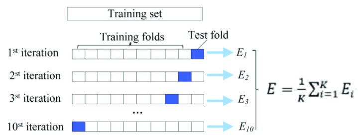
In order to simplify the process of stratification of data and efficaciously partition it we also use StratifiedShuffleSplit.
\
Example: class sklearn.model\_selection.StratifiedShuffleSplit(n\_splits=10, \*, test\_size=80%, train\_size=20%, random\_state=None)
Traditionally for classification model evaluation, confusion matrix is used. The basic principle of confusion matrix is to visualize the system confusing two classes. In our case, the confusion matrix can be appropriately used in order to ascertain whether the prediction mechanism is working as intended. Each instance in the confusion matrix is represented by two classes: actual and predicted. In this vein we can train the system to more accurately predict a particular address' likelihood of being fraudulent, in other words, increase specificity and consistency.
*eval <- evaluate(d\_binomial,*
*target\_col = "target",*
*prediction\_cols = "prediction",*
*type = "binomial")*
*eval*
*#> # A tibble: 1 x 19*
*#> \`Balanced Accuracy\` Accuracy F1 Sensitivity Specificity \`Pos Pred Value\`*
*#> \ \ \ \ \ \*
*#> 1 0.551 0.58 0.672 0.632 0.469 0.717*
*#> # … with 13 more variables: Neg Pred Value \, AUC \, Lower CI \,*
*#> # Upper CI \, Kappa \, MCC \, Detection Rate \,*
*#> # Detection Prevalence \, Prevalence \, Predictions \,*
*#> # ROC \, Confusion Matrix \, Process \*
*conf\_mat <- eval$\`Confusion Matrix\`\[\[1]]*
*conf\_mat*
*#> # A tibble: 4 x 5*
*#> Prediction Target Pos\_0 Pos\_1 N*
*#> \ \ \ \ \*
*#> 1 0 0 TP TN 15*
*#> 2 1 0 FN FP 17*
*#> 3 0 1 FP FN 25*
*#> 4 1 1 TN TP 43*
The basic calculation then will look in the following way: 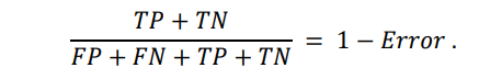
True positives are data points labeled as positive that are actually positive whereas false positives are data points labeled as positive that are actually negative. True negatives are data points labeled as negative that are actually negative whereas false negatives are data points labeled as negative that are actually positive.
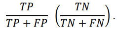
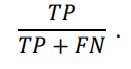
As a standard for classification method we will use metrics such as F1-score, precision, and recall. Instead of giving preponderance to either recall or precision, we use F1-score to essentially combine them into one metric. Precision in our case examines specifics of one class. For instance it would mean that the model will become better at predicting the fraudulence of a given transaction/address rather than non-fraudulence. In general, Recall metric refers to the extraction of a correctly predicted result by the model. Therefore, the Recall metric can be deemed to be a kind of purveyor of data points of interest.
The use of different methods for classification will allow us to yield far more reliable results and train our model to achieve higher specificity and accuracy. One of the models that will help us to build an efficient classification model is Random Forest. The gist of Random Forest has arbitrarily selected k features from the total m features, in cases where k < m. The Random Forest randomly selects k features from m total features, where k < m. From the entirety of k features, it calculates the node point d by alluding to the best splitting spot. Afterward, the nodes are divided into smaller nodes, again by using the splitting spot. In general, this iterative process is executed until l number of nodes has been reached. The Random Forest is built by reiterating the same process n number of instances and creating n number of trees. The results are obtained by the modal value of categories obtained by individual trees.
The main hurdle in establishing a fully working machine learning model is to train it on as much as possible a diverse set of scenarios. In the case of fraudulent transactions and their not as prolific (fortunately) scope, a case can be made that a system or model created on the sparse set of scenarios may not glean a sufficiently adequate result. This can partially be remedied with the help of historically available data on fraudulence as well as pre-imputed datasets. We also resort to the binary classification model for the time being as it allows us to minimize the computational overhead and simplify the model for the very first iteration while in the database-building phase.